

Closing the loop at a pumping station
At a variable-speed pumping station the operator asks for 5 bar. A pressure transmitter on the discharge pipe reads 3 bar. The PLC reads the measurement and calculates the error e = r − y = 5 − 3 = +2 bar. The controller uses the error and its internal state to calculate a command u within 0–100%. The variable-frequency drive (VFD) converts that command into a speed reference subject to its own limits. Pump speed and discharge pressure change. The PLC reads pressure again at its next sample, and the cycle repeats.
VFD and motor Process
pump and piping
In this operating region, increasing speed raises pressure at a fixed flow. A positive error therefore calls for more command. Consumer demand affects the process independently of the drive command. When demand rises, the pressure drop prompts the controller to respond through feedback.
Proportional action and steady-state error
With Kp = 10%/bar and a pressure error of +2 bar, the proportional contribution is +20 percentage points. It contributes to the calculated output alongside any bias and other terms. A higher Kp gives a stronger reaction to the same error. With phase lag, the same gain increase can produce oscillation and reduce the stability margin.
Consider a stable loop with unity negative feedback, a process with positive static gain K, zero bias, a constant setpoint and an unsaturated P controller. The steady-state process equation is y = Ku.
- The controller gives u = Kp·e.
- Substituting into the process equation gives y = K·Kp·e.
- Substitute into e = r − y and collect the error terms.
For K = 0.1 units/%, Kp = 10%/unit, and r = 5 units, the denominator is 2. The error is 2.5 units, the measurement is 2.5 units, and the command is 25%. The self-regulating process needs that nonzero command to hold the operating point. An unbiased P controller supplies it while an error persists.
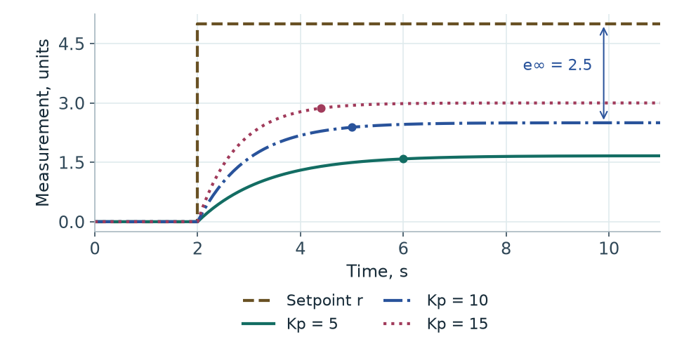
| Kp, %/unit | Reading, units | Error, units | t₉₅, s |
|---|---|---|---|
| 5 | 1.67 | 3.33 | 4.0 |
| 10 | 2.50 | 2.50 | 3.0 |
| 15 | 3.00 | 2.00 | 2.4 |
The table gives the steady reading and error. t₉₅ measures the time from the step to 95% of each response’s own final value. These runs never enter a narrow settling band around the 5-unit setpoint. The observed speedup applies to this model at L = 0. Dead time and actuator saturation can change the shape of the response.
Integral action and reachable setpoints
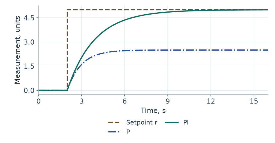
The integrator accumulates signed area under the error curve. Positive error increases I, negative error decreases it, and zero error holds its current value. This lets a PI controller supply the command needed at equilibrium. The loop must remain stable and the target must be reachable. Excessive Ki can build a large correction before the process responds, leading to overshoot, oscillation or extended saturation.
Consider a teaching example in which 5 bar at a given demand takes a 50% command. A 40% upper drive limit makes that target unreachable. In the simplified static curve p∞ = max(0, 24·(u/100)² − 1) bar, 24 bar is the shut-off head at full speed and 1 bar is the loss at the selected demand. The curve gives 5 bar at 50% and 2.84 bar at 40%. Changing Ki affects how quickly I builds up. The permitted command remains 40%.
Derivative action and filtering
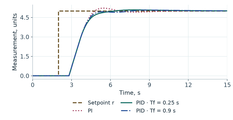
Two readings can have the same error while approaching the target at different speeds. D reacts to the rate of change. A quickly rising measurement produces a negative contribution when the controller differentiates the measurement. This can reduce overshoot and oscillation for a given process and set of gains.
When the controller differentiates the error, de/dt = dr/dt − dy/dt. A reference step enters D directly. In the sampled calculation, the step size is divided by Ts and causes a sharp change in command called derivative kick. Differentiating the measurement removes the direct contribution of changes in r to D. P and I still use the error.
Measurement noise can produce rapid changes in the reading even when the process is nearly stationary. A first-order filter with time constant Tf limits high-frequency gain compared with an ideal differentiator. A larger Tf smooths D further and adds lag to this branch. PI is often a practical choice for pressure control when a noisy measurement makes D costly and PI already meets the performance target.
Gains and PID forms
| Parameter | Main effect | Potential problems |
|---|---|---|
| Kp | Changes the strength of the response to the current error | Oscillation and reduced stability margin |
| Ki | Removes persistent error in a stable loop at a reachable target | Overshoot and integrator windup |
| Kd | Responds to the rate of change of the measurement | Sensitivity to measurement noise |
| Tf | Filters the D branch | Extra lag in derivative action |
These are typical effects. The response depends on process gain, inertia and dead time, the sample interval, measurement range, and actuator behaviour near its limits.
In the parallel form used by PID Lab, the pre-limit command is u = b + P + I + D*. With u in percent and the measurement in engineering units, Kp has units of %/unit, Ki of %/(unit·s), and Kd of %·s/unit. Tf and Ts are in seconds. In the form with a common gain, Kp scales all terms, Ti is the integral time and Td is the derivative time.
For Kp > 0, the inverse gives Ti = Kp/Ki for Ki > 0, and Td = Kd/Kp. Integral action is disabled at Ki = 0, the limit Ti → ∞. If a standard filtered form uses a divisor N > 0, its filter time is Tf = Td/N for Td > 0. Equivalent gains require the same inputs to P, I and D and the same discretisation. Check the parameterisation of the particular PLC block.
Output limits and anti-windup
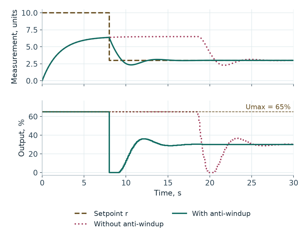
Suppose a drive accepts up to 100%, and the controller calculates u = 130%**. The limited command is u = 100%. Without protection, positive error keeps increasing the integral. A drop in demand or in the setpoint can reverse the error. The command can still stay at its maximum until negative error has reduced the accumulated I enough for u to return to range.
- Conditional integration. Block the integral increment in the direction of saturation, or cap it at the remaining headroom. Allow increments that bring the command out of saturation. PID Lab caps the increment in its direction of change.
- Back-calculation. Add (u − u)/Tt* to the rate of change of the integral, where Tt > 0 is the back-calculation time. At upper saturation this term is negative and unwinds the integral. Tt affects both the recovery speed and behaviour near the limit.
- Tracking. Align controller state with an applied command utr. This can be a manual command, selector output, or rate-limited drive reference. Tracking can set the state directly on a mode change or use a feedback correction. Bring an external limit back to the controller in compatible units.
Bumpless transfer from manual to auto
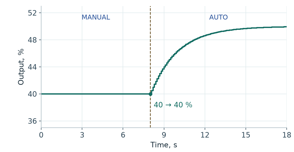
In MANUAL, the operator sets the command. In AUTO, the controller calculates it. When switching to AUTO, a mismatch between the manual command and the sum of P, I, and D can cause a command step. With bumpless transfer, the first automatic sample holds the applied manual command within the actuator’s limits.
This equation assumes no separate bias, an available integrator, and P and D evaluated at the current sample. Subtract a fixed bias b as well if it is present. With I disabled, the controller can align a tracking bias instead. Initialise and update the previous measurement and the derivative filter, including while in manual. If limits change or the actuator has a rate limit, base tracking on a command the actuator can actually apply.
In the PI example with a 40% manual command, the reading at t = 8 s is about 3.927 units for a 5-unit setpoint. At that sample P ≈ 10.73%, D = 0, and I ≈ 29.27% gives the tracking value. The first automatic sample holds 40%. On the next sample, the command moves to 40.50% in response to the remaining error.
Discrete implementation in a PLC
Ts is the interval between controller calls. The states in a continuous model change continuously. A PLC reads the measurement, updates its states, and writes the output at sample times. The command is typically held between calls. Execute the block once per cycle in a predictable periodic task. Passing a nominal Ts to code with a significantly varying interval changes the effective action of I and D.
Backward Euler integrates the current error sample. Anti-windup can cap ΔIₖ before the update Iₖ = Iₖ₋₁ + ΔIₖ.
For the D filter, replace both derivatives with differences between k and k−1 and solve for D at the current sample. With positive Tf and Ts the memory coefficient Tf/(Tf + Ts) is between 0 and 1.
Teaching function block in Structured Text
Pass SP and PV in the same engineering units. Ts and Tf are in seconds. Umin, Umax, Umanual, and U are in percent. ManualMode selects the calculation branch. Set Kd = 0 for PI, and Ki = Kd = 0 for P. Set gains before starting and keep them fixed for the run.
On the first valid cycle the block copies PV into PrevPV, so D starts from zero. A manual start applies the limited manual command. On automatic startup, integration begins with the first sample. At transfer from manual, that sample aligns the internal state. Invalid parameters clear ConfigOK, hold the last command and reset the internal states. A subsequent valid configuration starts with initialisation. The calling program decides the safe actuator output. In CODESYS place the declaration beginning at FUNCTION_BLOCK in the POU declaration area and the body up to END_FUNCTION_BLOCK in the implementation area.
FUNCTION_BLOCK FB_PidTeaching
VAR_INPUT
    SP, PV : LREAL;
    Kp, Ki, Kd : LREAL;
    Ts, Tf : LREAL;
    Umin, Umax, Umanual : LREAL;
    ManualMode : BOOL;
END_VAR
VAR_OUTPUT
    U : LREAL := 0.0;
    ConfigOK : BOOL;
END_VAR
VAR
    Initialized, WasManual : BOOL;
    PrevPV, Err, P, Ipart, D, Bias : LREAL;
    BeforeI, DeltaI : LREAL;
END_VAR

ConfigOK := (Ts > 0.0) AND (Tf > 0.0)
    AND (Kp >= 0.0) AND (Ki >= 0.0) AND (Kd >= 0.0)
    AND (Umin >= 0.0) AND (Umax <= 100.0) AND (Umin < Umax);

IF NOT ConfigOK THEN
    Initialized := FALSE;
    WasManual := FALSE;
    Ipart := 0.0;
    D := 0.0;
    Bias := 0.0;
    RETURN;
END_IF;

IF NOT Initialized THEN
    PrevPV := PV;
    D := 0.0;
    Initialized := TRUE;
END_IF;

Err := SP - PV;
P := Kp * Err;
D := (Tf * D - Kd * (PV - PrevPV)) / (Tf + Ts);
PrevPV := PV;

IF ManualMode OR WasManual THEN
    IF ManualMode THEN
        U := LIMIT(Umin, Umanual, Umax);
    ELSE
        U := LIMIT(Umin, U, Umax);
    END_IF;

    IF Ki > 0.0 THEN
        Ipart := U - P - D;
        Bias := 0.0;
    ELSE
        Ipart := 0.0;
        Bias := U - P - D;
    END_IF;
ELSE
    BeforeI := P + Ipart + D + Bias;
    DeltaI := Ki * Ts * Err;

    IF DeltaI > 0.0 THEN
        DeltaI := MIN(DeltaI, MAX(0.0, Umax - BeforeI));
    ELSIF DeltaI < 0.0 THEN
        DeltaI := MAX(DeltaI, MIN(0.0, Umin - BeforeI));
    END_IF;

    Ipart := Ipart + DeltaI;
    U := LIMIT(Umin, P + Ipart + D + Bias, Umax);
END_IF;

WasManual := ManualMode;
END_FUNCTION_BLOCKThree industrial applications
Discharge pressure
A pumping station measures discharge pressure, adjusts VFD frequency, and experiences changes in consumer flow as disturbances. In a region with positive process gain, higher demand increases losses and lowers pressure. PI responds by increasing speed. With sufficient speed available, I restores pressure after a sustained demand change. The simplified PID Lab model includes pressure lag and losses proportional to the square of flow. Its pump experiment changes demand from 2 to 4 m³/h at a 4 bar setpoint.
Minimum and maximum frequency, acceleration limits, and measurement delay all affect reachability and dynamics. High gain with appreciable dead time can lead to repeated acceleration and deceleration. A stable PI loop can reject sustained changes in demand. Its response and measurement noise determine whether adding D is worthwhile.
Tank level
For a tank with constant cross-sectional area A and flow rates in m³/s, A·dh/dt = Qin − Qout away from the boundaries. Level holds when flows balance. A persistent imbalance keeps level moving, so this is an integrating process. When demand rises, the controller opens the inlet valve until the added flow is supplied. The lab model limits discharge by available water and accounts for excess volume as overflow.
For A = 0.4 m², an outlet flow increase of 15 m³/h with the same inflow changes the level slope by −15/(3600·0.4) ≈ −0.0104 m/s. A self-regulating pressure model approaches another equilibrium for a fixed command and demand. An unbalanced tank continues towards a capacity boundary. Tune level control around acceptable level excursions and the available time before overflow or dry-out. An overly active loop can pass flow variations on to neighbouring processes.
Industrial furnace temperature
Near an operating point, a furnace can be approximated by C·dθ/dt = η·Pmax·u(t−L)/100 − H·(θ−θa) − Qload. Here C is effective heat capacity in J/K, H is the heat-loss coefficient in W/K, θa is ambient temperature, η·Pmax is the available heating power, and Qload is heat drawn by the product. Dead time L approximates heat transport and measurement delays. For H > 0, the linear model has T = C/H and a static gain K = η·Pmax/(100·H) in kelvins per percentage point of command. A real furnace can have different heater, air and product temperatures, so a single time constant approximates only a chosen operating region.
On heat-up, the heater can spend a long time at its limit. High Ki can build up a large correction before the sensor registers enough heat. Due to dead time, the reading can keep rising for a while after power is reduced. Evaluate warm-up, disturbances from loading, power limits and the margin to maximum temperature. PID Lab provides a generic first-order process and dead-time experiments. The furnace here is a separate calculation example.
Check your understanding
Why can a P controller have a steady-state error?
With no bias, a nonzero steady command requires an error because u = Kp·e. For the example it is r/(1 + K·Kp) under the stated conditions.
Why does increasing Ki fail to reach an infeasible setpoint?
The integral raises the calculated sum. The actuator is constrained and continues applying the maximum permitted command.
What does anti-windup do?
It limits integration when the actuator is saturated or aligns the state with the applied command. This improves recovery when conditions change.
How does derivative on measurement differ from derivative on error?
Error contains both reference and measurement changes. Differentiating measurement removes the direct contribution of a reference step to D.
Why does PID need predictable task timing?
The I increment and D filter are calculated for Ts. Irregular calls change their effective behaviour over time.
What makes a transfer bumpless?
The first sample after a mode change holds the applied command within the actuator limit. The controller adjusts its internal state to match the command.
When is PI enough?
When PI meets the performance target across operating points and disturbances, and D offers little improvement or reacts too strongly to noise.
Practical takeaways
Start with controller direction, engineering units, and a reachable setpoint. Compare both measurement and applied command under matching conditions. Include recovery from saturation, manual-to-auto transfer, and load changes in the trials. Add D when its benefits hold at representative dead time and noise. Before transferring the design to a PLC, set the task period, verify units and test the process protections separately.